估计

大模型训练需要多少GPU？大模型显存怎么算？ #大模型 #AI系统

大模型推理需要多大的显存？ #大模型 #AI系统 #推理 #显存

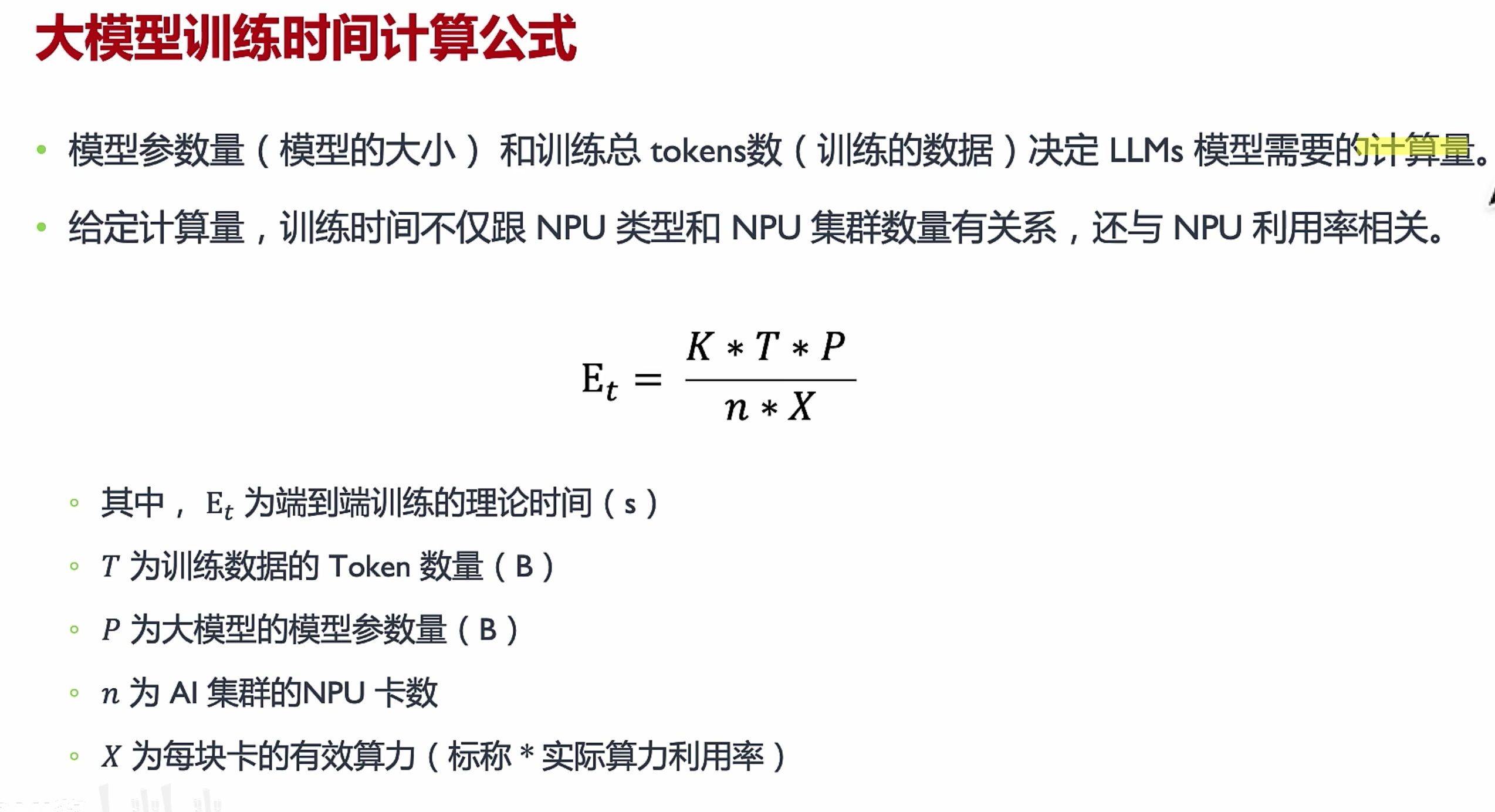
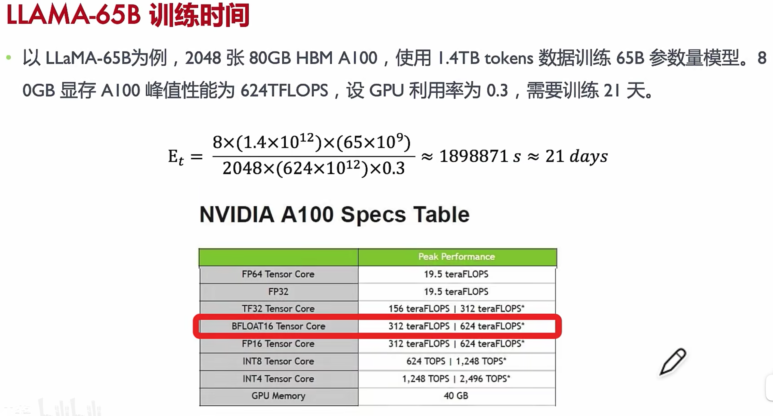
训练时间估计

训练显存

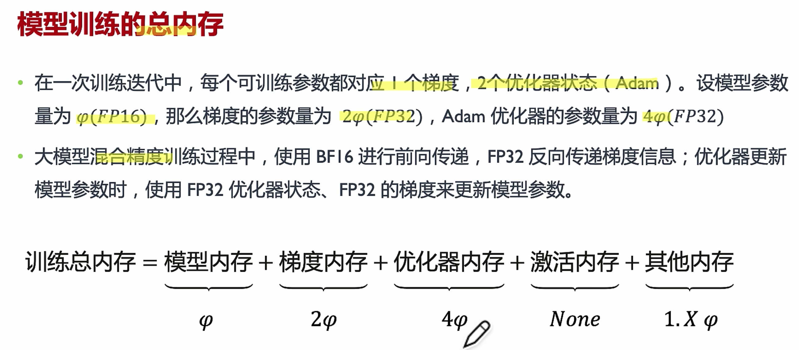
优化器内存=一阶动量+二阶动量，所以2+2=4，参数大小FP16加载的话= 权重大小B*2Byte 约定于6B模型占12G显存，训练至少是这个值8倍。

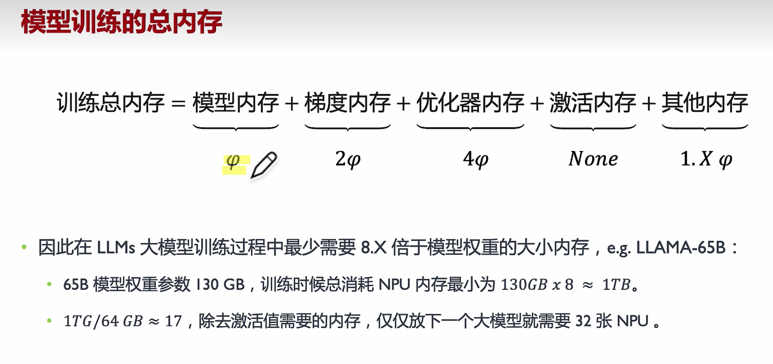
不能是17张卡，要8的倍数（分布式训练一个节点8张卡），而且激活值用于反向传播计算梯度用，占的是大头显存。所以真正用到会更多

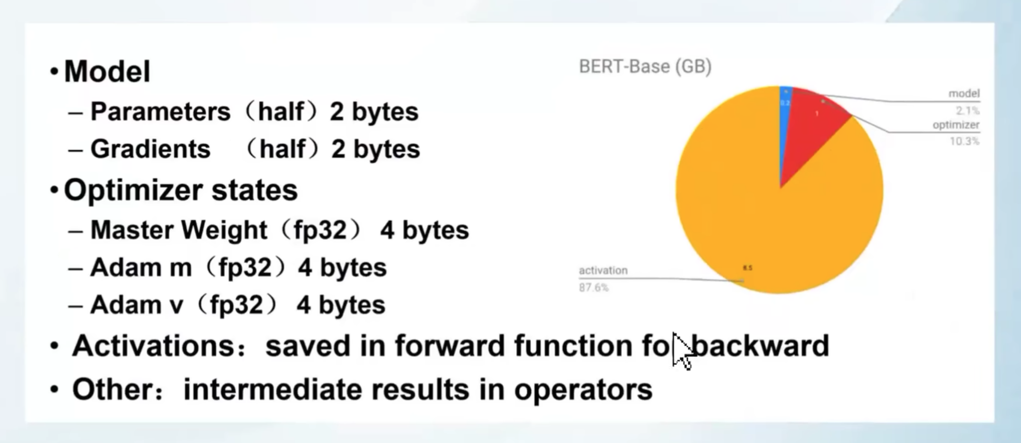
占用计算 1B（十亿参数）的模型 , float 4字节 half 2Byte

参数量 = 1B * half = 2GB

梯度 = 1B * half = 2GB

优化器= 1B * 8Bytes（AdamW） = 8GB

还有其他等等（激活函数也需要占据额外的显存，其随批量大小（batch size）和序列长度而增加）

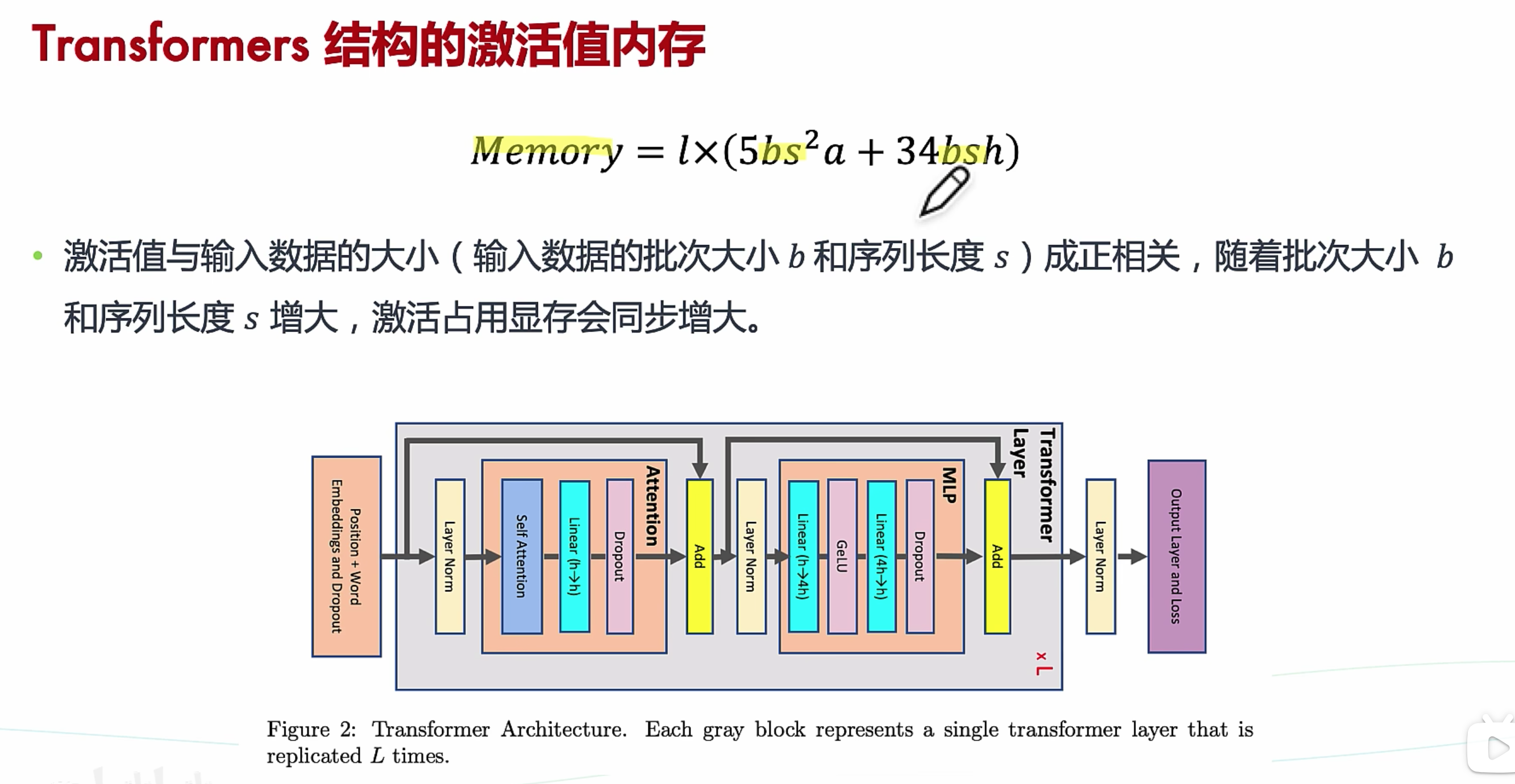
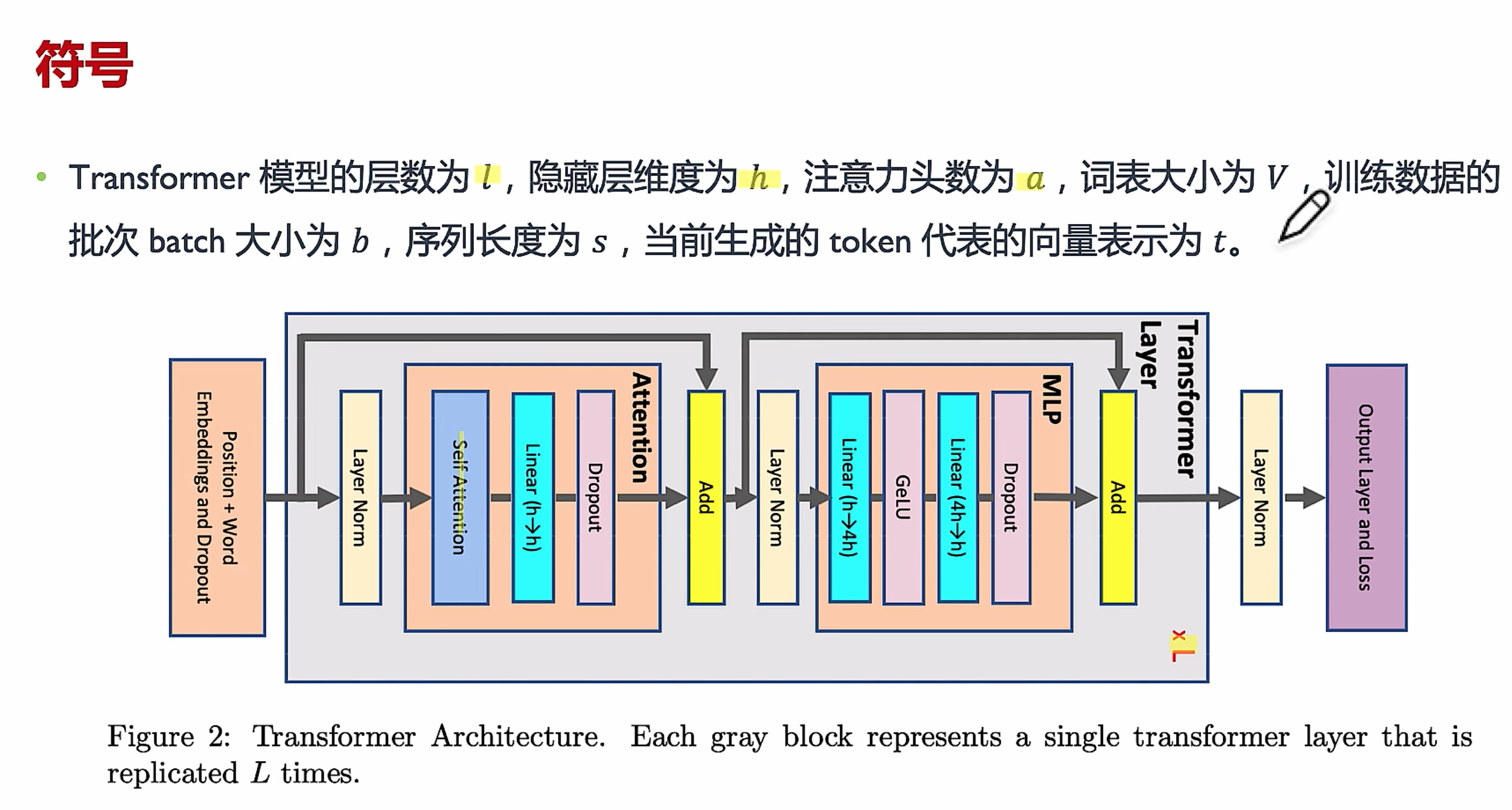
block 的层数l，a为注意力头数，隐藏层数h。

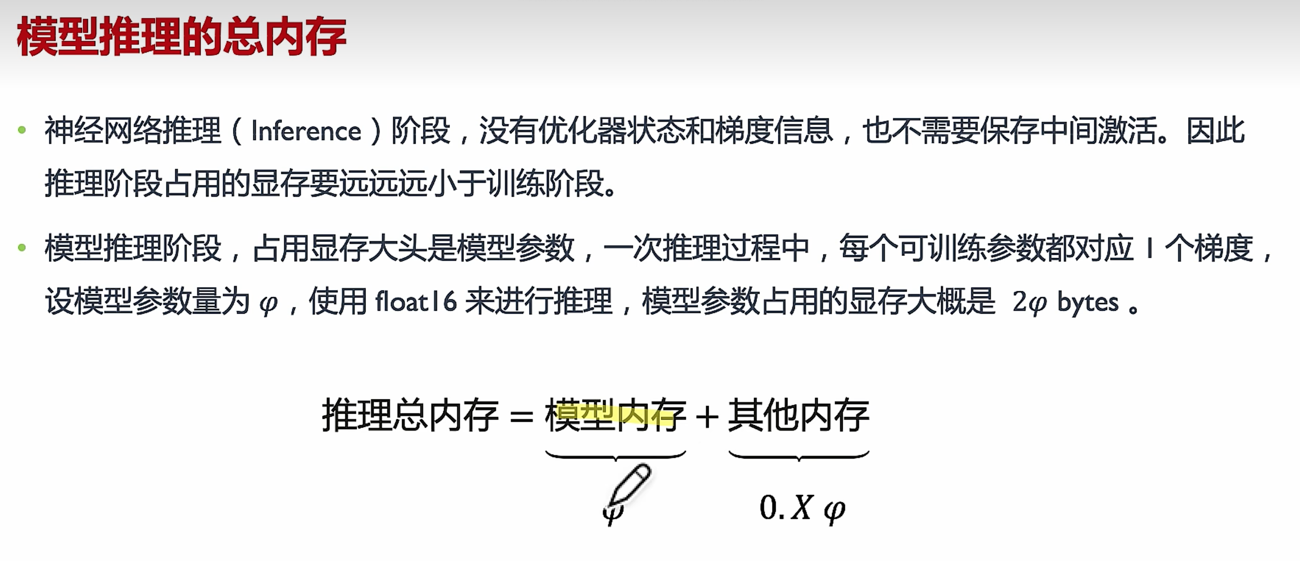
推理显存

大概两倍模型显存大小=2*模型规模B*2Byte

目前流行的使用KVcache，推理尽可能单卡，减少通信，主要用GDDR进行推理加速，HBM用在训练。

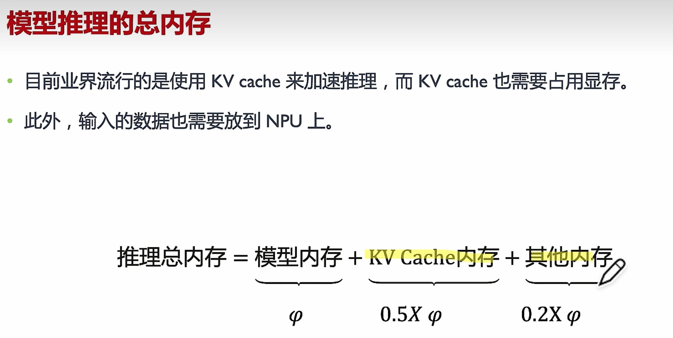
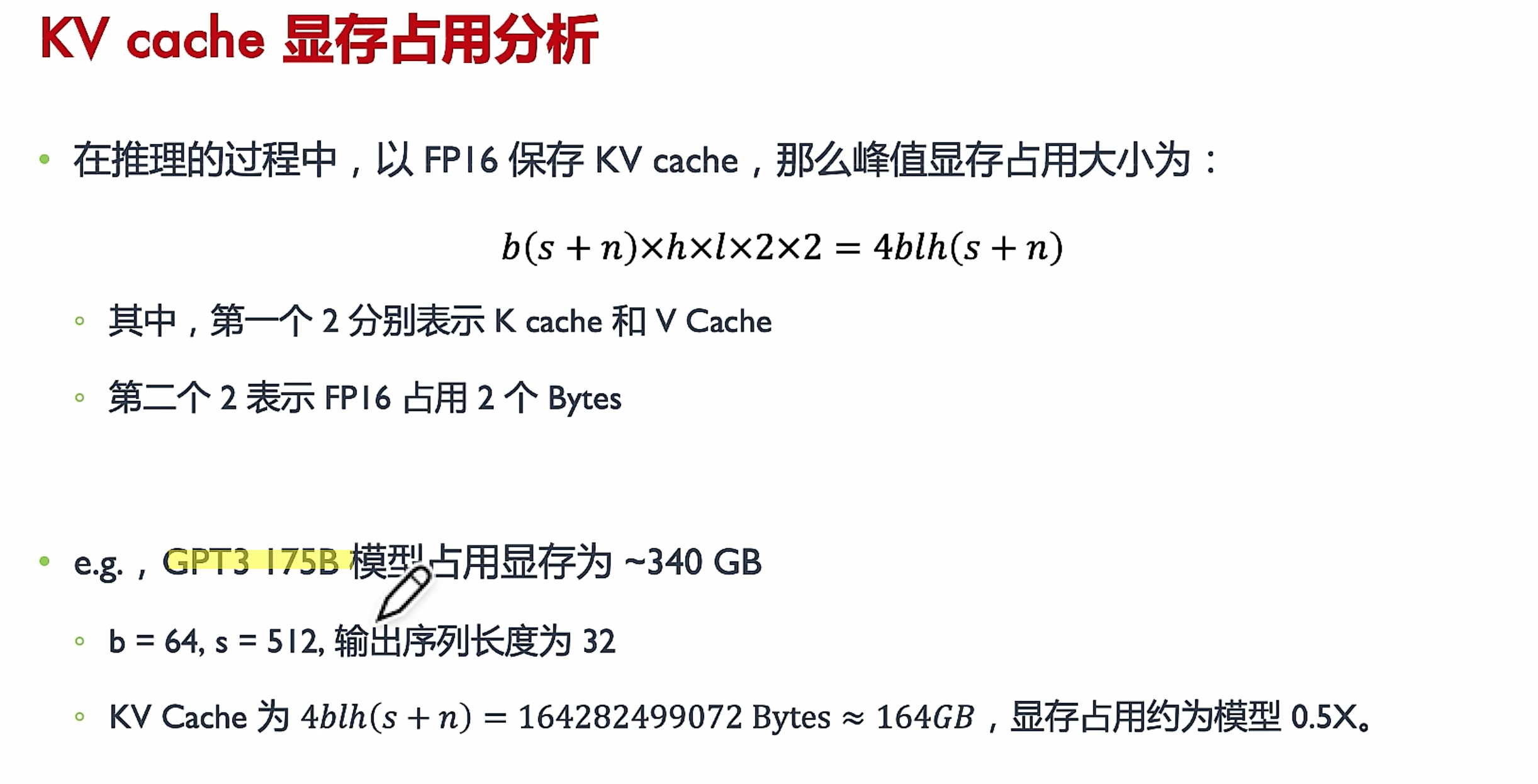
kv cache 显存占用

节省显存，内存

调节训练参数

占用计算 1B（十亿参数）的模型 , float 4字节 half 2Byte

参数量 = 1B * 4Bytes = 4GB

梯度 = 1B * 4Bytes = 4GB

优化器= 1B * 8Bytes（AdamW） = 8GB

还有其他等等（激活函数也需要占据额外的显存，其随批量大小（batch size）而增加）

# 参数量
sum(param.numel() for param in model.parameters())

节约显存，增大训练时间，可能也会影响训练效果

train_args = TrainingArguments(output_dir="./checkpoints",      # 输出文件夹
                               per_device_train_batch_size=1,   # 训练时的batch_size
                               gradient_accumulation_steps=32,  # *** 梯度累加 ***
                               gradient_checkpointing=True,     # *** 梯度检查点 ***
                               optim="adafactor",               # *** adafactor优化器 *** 
                               per_device_eval_batch_size=1,    # 验证时的batch_size
                               num_train_epochs=1,              # 训练轮数
                               logging_steps=10,                # log 打印的频率
                               evaluation_strategy="epoch",     # 评估策略
                               save_strategy="epoch",           # 保存策略
                               save_total_limit=3,              # 最大保存数
                               learning_rate=2e-5,              # 学习率
                               weight_decay=0.01,               # weight_decay
                               metric_for_best_model="f1",      # 设定评估指标
                               load_best_model_at_end=True)     # 训练完成后加载最优模型

降低batch_size（一次梯度更新用的数据条数），造成训练效果降低，gradient_accumulation_steps（多少次batch后，才进行梯度更新）。gradient_accumulation_steps相应增加对应的batch_size减少的数量，可以保证训练效果，降低显存占用。
gradient_checkpointing=True，通过以更长的计算时间为代价，换取更少的显存占用。原本需要存储所有中间变量以供反向传播使用，使用了checkpoint不存储中间变量而是在反向传播过程中重新计算这些中间变量。（选择性保存中间结果）

开启报错的话
1
model.enable_input_require_grads() # 开启梯度检查点时，要执行该方法`
使用显存占用更少的优化器

参数冻结，只训练全连接层。

# *** 参数冻结 *** 
for name, param in model.named_parameters():
    param.requires_grad = False

加载参数

加载参数说明

使用device_map="auto"，Accelerate 将确定每个层的放置位置，以最大限度地利用最快的设备 (GPU)，并卸载 CPU 上的其余部分，如果没有足够的 GPU RAM（或 CPU RAM），甚至可以卸载硬盘驱动器。即使模型分布在多个设备上，它也会按照您通常的预期运行。

When using device_map="auto", Accelerate will determine the placement of each layer to maximize the utilization of the fastest device (GPU) and offload the rest onto the CPU, or even unload onto the hard drive if there is not enough GPU or CPU RAM. Even if the model is distributed across multiple devices, it will run as expected according to your usual expectations.

当传递 , 时device_map，low_cpu_mem_usage会自动设置为True，因此您无需指定它

 # 加载模型，device_map='auto' ，设置了device_map，默认low_cpu_mem_usage=True
  self.model = AutoModelForCausalLM.from_pretrained(self.model_id,
                                                          torch_dtype=torch.float16, # 
                                                          trust_remote_code=True,
                                                          low_cpu_mem_usage=True, device_map='auto')
  # 查看模型是如何跨设备分割
  self.model.hf_device_map

以前加载预训练的权重（需要模型两倍大小的内存，一个用于随机初始化的模型，一个用于权重），low_cpu_mem_usage=True使得创建模型时候为空模型，当加载权重时候才初始化，这样使用的最大内存仅为模型的完整大小。

By setting low_cpu_mem_usage=True, the model will be created as an empty model during initialization, without any preloaded weights. This helps to reduce the memory usage to only the size of the complete model when loading pretrained weights. In other words, the maximum memory used will be limited to the size of the model itself. This approach allows for more efficient memory utilization when working with pretrained weights.

降低精度

要看显卡对精度(precision)的支持

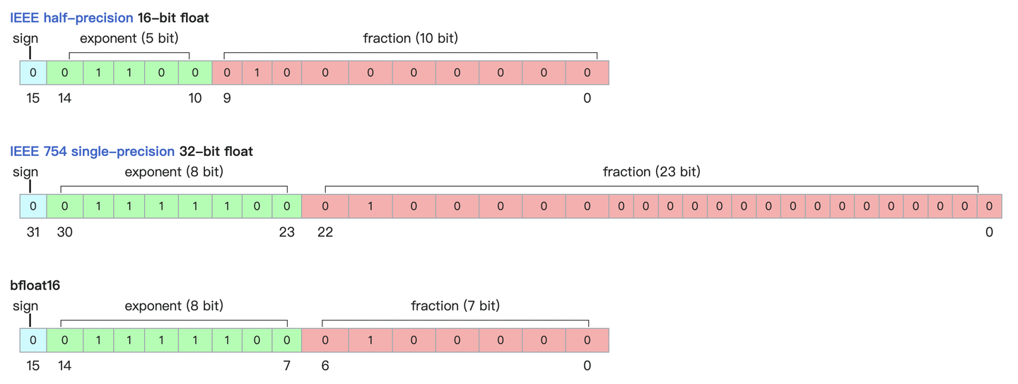
当然也可以使用量化模型(Quantized model)，或者更低精度（加载模型时候使用torch_dtype，一般加载用torch.float16或者torch.bfloat16）。通常用BF16 （精度低，范围大），因为FP16（half, 半精度,精度高）会经常溢出，导致数值不稳定、模型不收敛(non-convergence) ，新卡支持BF16

It is common to use the BF16 (bfloat16) data type because it offers a larger range while maintaining a lower precision. This can be beneficial in avoiding frequent overflow issues that may arise with the FP16 (half precision) data type, which can lead to numerical instability and non-convergence of the model. It’s great to know that the new cards support BF16, as it provides a good balance between precision and range for improved model stability and convergence.

符号位，指数位（取值范围），尾数(精度)

精度对模型的影响

浮点数据类型主要分为双精度（FP64）、单精度（FP32 1 8 23）、半精度（FP16）BF16，int8 , fp4，nf4

深度学习模型训练好之后，其权重参数在一定程度上是冗余的，在很多任务上，我们可以采用低精度

好处

减少内存，显存，存储占用：FP16的位宽是FP32的一半，因此权重等参数所占用的内存也是原来的一半，节省下来的内存可以放更大的网络模型或者使用更多的数据进行训练。Memory Reduction: FP16 has half the bit width of FP32, meaning that the memory occupied by weights and other parameters is also reduced by half. This frees up memory that can be used to accommodate larger network models or train with more data.
加快通讯效率：针对分布式训练，特别是在大模型训练的过程中，通讯的开销制约了网络模型训练的整体性能，通讯的位宽少了意味着可以提升通讯性能，减少等待时间，加快数据的流通。Improved Communication Efficiency: In distributed training, especially with large models, communication overhead can significantly impact overall performance. With a narrower bit width for communication, the efficiency of data transmission is improved, reducing waiting time and accelerating data flow.
计算效率更高：使用FP16的执行运算性能比FP32更加快 Enhanced Computational Efficiency: FP16 computations can be performed faster compared to FP32, leading to improved computational efficiency.
降低功耗 Lower Power Consumption: With reduced precision, FP16 computations generally consume less power compared to FP32.
支持微处理器，有些微处理器属于8位的，低功耗运行浮点运算速度慢，需要进行8bit量化

可以让模型在边缘集群或终端机器运行。

坏处

精度损失，推理精度确实下降

低精度训练FP16

半精度LLama训练

LlaMA2模型分词器的padding_side要设置为right，否则可能不收敛
LlaMA2模型的分词器词表的问题要适当调整数据的最大长度，保证数护内容的完整性
LlaMA2模型加载时，torch_dtype为半精度，否则模型将按照fp32加载
当启用gradient_checkpoint训结时，需要一并调用model.enable_input_require_grads()方法
当完全采用fp16半精度进行训练且采用adam优化器时，需要调整优化器的adam_epsilon的值，否则模型无法收敛

int8

量化是一种模型压缩的方法，使用低精度数据类型对模型权重或者激活值进行表示。简单来说，量化就是将高精度的数字通过某种手段将其转换为低精度的数据

原理

absmax量化的细节。要计算absmax量化中fp16数字与其对应的int8数字之间的映射，您必须首先除以张量的绝对最大值，然后乘以数据类型的总范围。

例如，假设您想要在包含的向量中应用 absmax 量化[1.2, -0.5, -4.3, 1.2, -3.1, 0.8, 2.4, 5.4]。您提取它的绝对最大值，5.4在本例中就是如此。Int8 的范围为[-127, 127]，因此我们将 127 除以5.4并获得23.5缩放因子。因此，将原始向量乘以它就得到量化向量[28, -12, -101, 28, -73, 19, 56, 127]。

优化方法

使用更多的量化参数 (scale factor) Use more quantitative parameters
矩阵乘法（Matrix multiplication）A*B可以看作是A的每一行乘上B的每一列（column），为A的每一行和B的每一列单独设置scale factor，这种方式被称之为Vector-wise量化 For each row of A and each column of B, set a separate scale factor. This approach is called Vector-wise quantization.
离群值（Outliers）: 超出某个分布范围的值通常称为离群值。8 位精度的动态范围极其有限，因此量化具有多个大值的向量会产生严重误差。误差在一点点累积的过程中会导致模型的最终性能大幅度下降 Values that are outside a certain distribution range are usually referred to as outliers. With a limited dynamic range of 8-bit precision, quantizing vectors with multiple large values can result in significant errors. The accumulation of errors over time can greatly degrade the final performance of the model.

使用

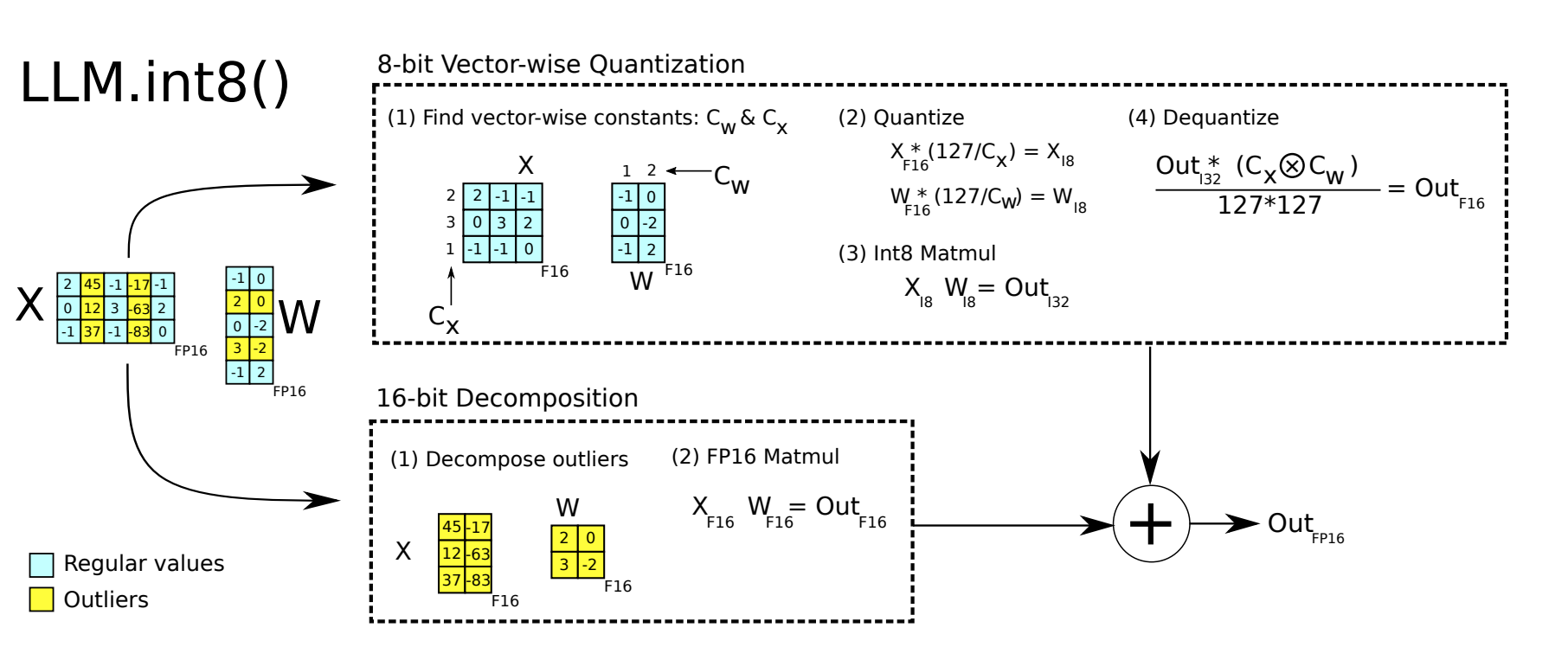
从输入隐藏状态中，按列提取异常值（即大于特定阈值的值） Extracting outliers (values greater than a specific threshold) from the input hidden state column-wise.
对 FP16 中的离群值矩阵和 int8 中的非离群值矩阵分别执行矩阵乘法 Performing matrix multiplication on the outlier matrix in FP16 and the non-outlier matrix in int8.
对非离群值矩阵结果进行反量化，并将离群值和非离群值结果相加，以获得 FP16 中的完整结果。 Dequantizing the result of the non-outlier matrix and adding it to the outlier matrix to obtain the complete result in FP16.

model = AutoModelForCausalLM.from_pretrained("xxxxx", trust_remote_code=True, low_cpu_mem_usage=True, 
                                             torch_dtype=torch.half, device_map="auto", load_in_8bit=True)

# 主要改造矩阵乘法，是int8,fp16混合精度（混合精度）模型
for name, param in model.named_parameters():
    print(name, param.dtype)

int4

4bit 量化，不能继续使用线性量化，4 bit的表示范围比8bit更小，粒度更粗，不用非常大的离群值，就使得量化后的参数都集中在某数值上，量化误差会非常大

线性量化

数据归一化到[-1，1]，把[-1，1]均匀切分成N区间 (N取决于量化bit)，归一化的结果归属于第几个区间，量化结果便为几。

数据的分布对量化结果非常重要。如果待量化的数据为均匀分布，那么线性量化的结果即使是4bit也不会太差

但是一般模型权重数值分布，并不是均匀分布，而是正态分布。

def get_weights(model):
    weights = []
    for param in model.parameters():
        weights.append(param.view(-1))
    return torch.cat(weights)
weights = get_weights(model)
bins = 200
hist = torch.histogram(weights.float(), bins=bins, range=(-0.1, 0.1))

import matplotlib.pyplot as plt
import matplotlib.ticker as ticker
import numpy as np
x = range(bins)
plt.figure(figsize=(16, 9))
plt.bar(x, hist.hist.detach().numpy(), color="orange")
plt.xticks(x, np.linspace(-0.1, 0.1, 200).round(3))
plt.gca().xaxis.set_major_locator(ticker.MultipleLocator(10))

分位数量化

把顺序排列的一组数据分割为若干相等部分的分割点的数值即为相应的分位数。

四分位数则是将数据按照大小顺序排序后，把数据分割成四等分的三个分割点上的数值.

示例 {6, 7,15, 36, 39, 40, 41, 42, 43,47,49) 二分位数 (中位数): 40 四分位数:15，40，43

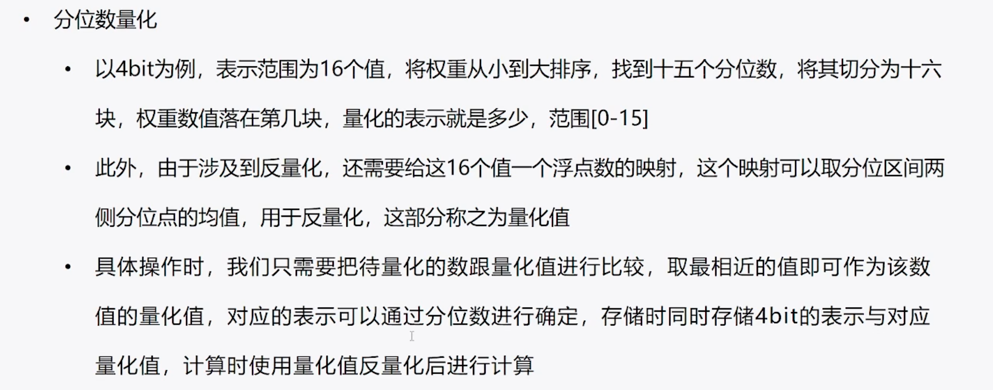
要存储的值非常多

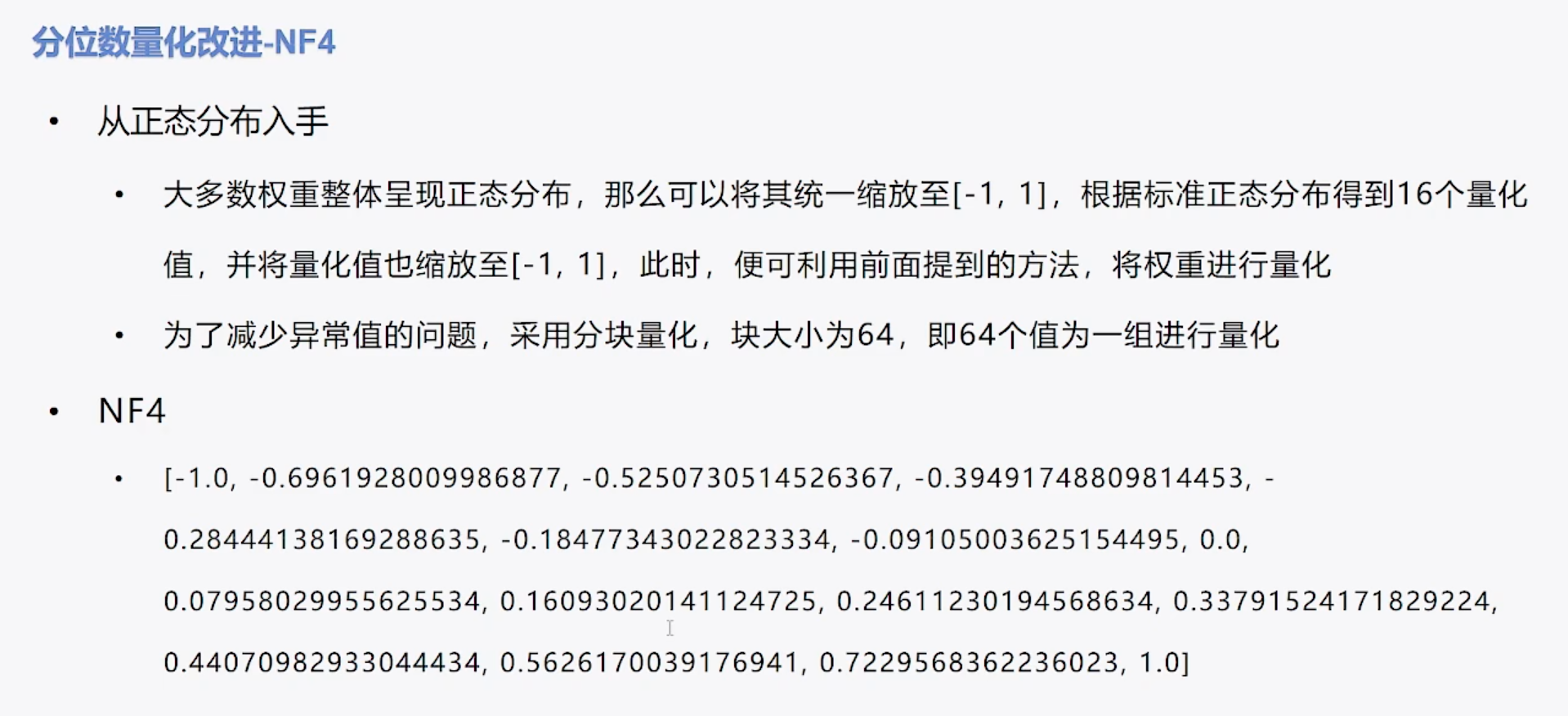
NF4算法

根据标准正态分布得到16个量化值，并将量化值也缩放至[-1，1]
Based on the standard normal distribution, I generated 16 quantized values and scaled them to the range of [-1, 1]

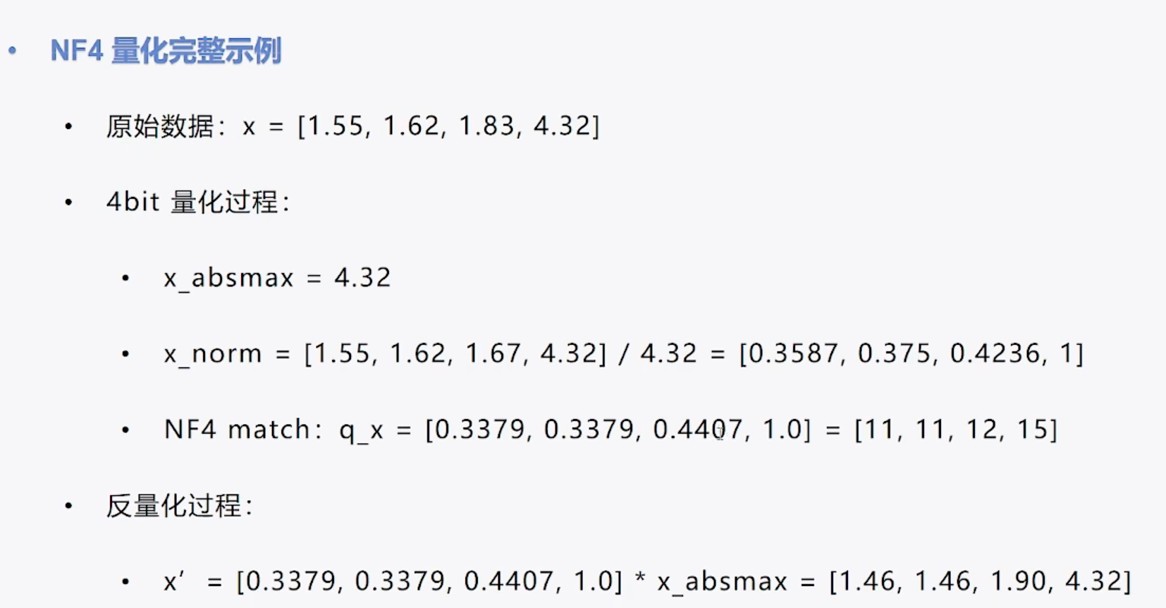
X_norm在NF4中找对应到对应量化值，q_x量化值对应index

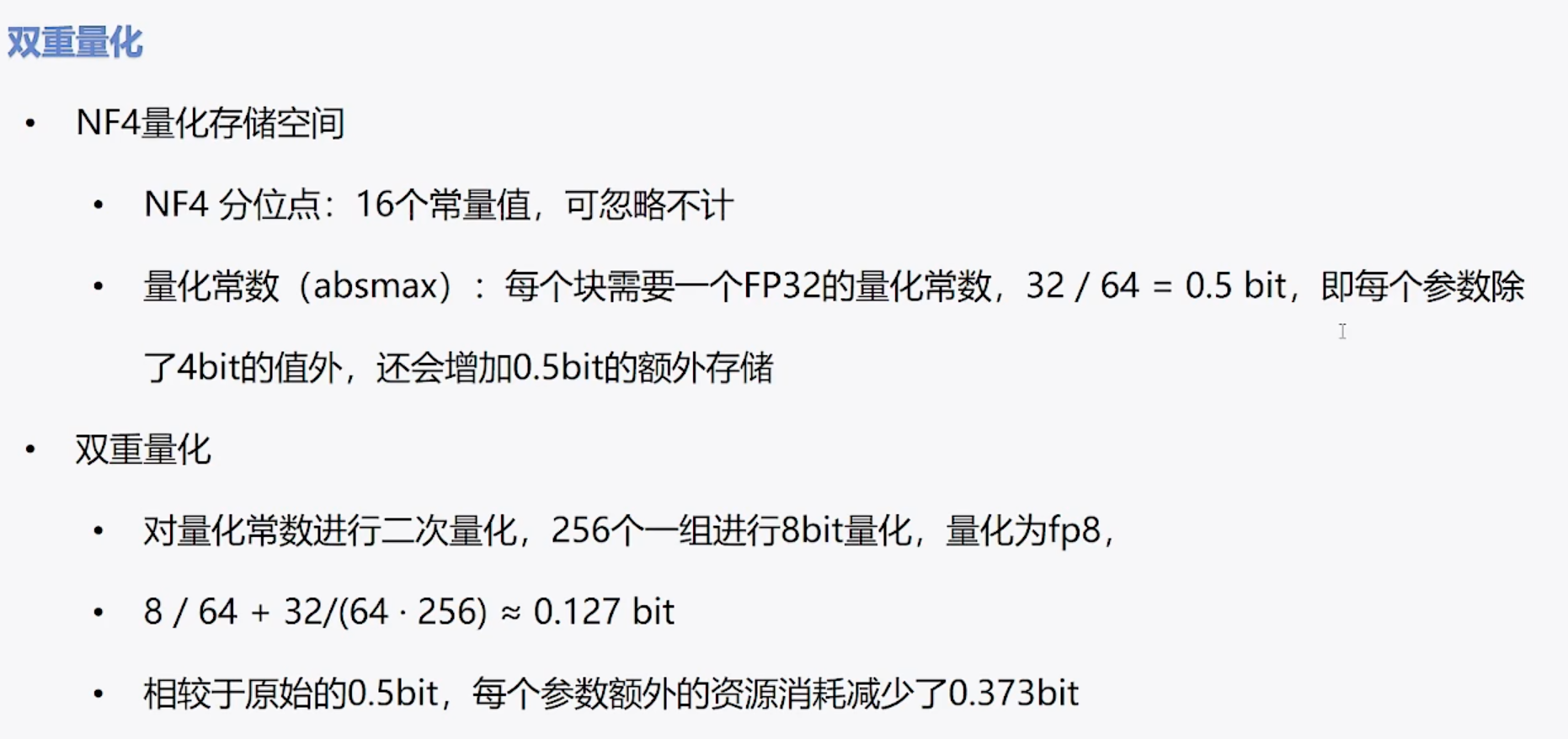
双重量化，减少存储空间，针对absmax，进行int8 double quantization to reduce storage space, using int8 for absmax.

分页优化器 当显存不足时，将优化器的参数转移到CPU内存上，在需要时再将其取回，防止显存峰值时OOM

model = AutoModelForCausalLM.from_pretrained("xxxxx", trust_remote_code=True, low_cpu_mem_usage=True, 
                                             torch_dtype=torch.half, device_map="auto", 
                                             load_in_4bit=True, # 核心
                                             bnb_4bit_compute_dtype=torch.half, # 4bit计算数值类型和torch_dtype一致
                                             bnb_4bit_quant_type="nf4",  # nf4 算法
                                             bnb_4bit_use_double_quant=True # 双重量化
                                            )

args = TrainingArguments(
    output_dir="./chatbot",
    per_device_train_batch_size=1,
    gradient_accumulation_steps=32,
    logging_steps=10,
    num_train_epochs=1,
    learning_rate=1e-4,
    remove_unused_columns=False,
    gradient_checkpointing=True,
    optim="paged_adamw_32bit" # 分页优化器
)

矩阵量化

per tensor(亦称layerwise)
- 整个矩阵看作集合S，矩阵中的所有元素共享一个缩放系数
- 优点在于简单，全局只有一个缩放系数
- 缺点也很明显，如果矩阵中数值尺度相差悬殊，那么大尺度的数值会导致一个很小的缩放系数，从而导致小尺度的数值趋于零甚至归零。而大语言模型常常具有这种数值分布特征，所以通常不使用per tensor，尤其是使用线形量化时。
per channel(亦称channelwise)
- 如果集合S内的数值波动越小，那么缩放系数就能越大，量化精度就越高。另一方面，如果S内的个数越少，出现大幅波动的概率也就越小，于是自然想到，将矩阵分片量化能提高量化精度，且分片越小，精度就越高。
- 将矩阵每一列作为一个分片进行量化，每一列内的所有元素共亨一个缩放系数，而列之间相互独立，这便是per channel量化，能增加数值之间的区分度，保留更多的源分布信息。
- 当然，按行分片也是可行的。在矩阵乘法AxB中，我们通常将A按行量化，将B按列量化，即原则上是沿着内维度(inner dimension)量化。换言之，假设A为MxK矩阵，B为KxN矩阵，则沿K维度量化，A有M个行缩放系数，B有N个列缩放系数。
- 在LLM中，A通常为activation，其每一行是某一个token的embedding，因此我们把A的按行量化也称为per token量化
groupwise
- 相对于分片，进一步提高精度。Groupwise是将G个元素看作集合S进行数值是化，G称为group size.
- 代价是缩放系数的个数膨胀，从per channel的N到 $\frac{M\times N}{group_size}$, 其中M为短阵行数，N为矩阵列数。
- 随着分片粒度变小，精度越来越高，而量化开销越大，这需要折衷，事实上，对于一个MxN的矩阵，per channel只是groupwise在group_size=M时的特例，per tensor则是group_size =MxN时的特例。

反量化

在构建模型时，各层的权重已经完成了量化。在推理过程中，根据activation是否使用量化数值类型，又可分为两大类weight-only，weiaht & activation。它们决定了短阵乘法过程中，反量化操作的执行时机

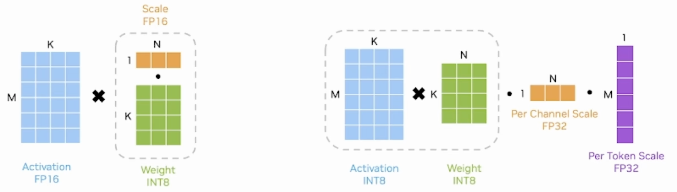
以典型的INT8 weight-only量化为例，其weight是per channel量化的INT8，而activation使用FP16类型。在推理时，需要先按列乘以scale将weight反量化为FP16，再与activation相乘
SmoothQuant方法是weight&activation量化，其weight和activation都使用INT8类型，所以有两组缩放系数，一组是用于wcight的per-channel scale，一组是用于activation的per-token scale。先执行INT8的矩阵乘法，再分别按列、按行乘以两组缩放系数

PEFT

Prompt tuning

原理

Prompt tuning peft 源码

from peft import PromptTuningConfig, get_peft_model, TaskType, PromptTuningInit

# Soft Prompt
config = PromptTuningConfig(task_type=TaskType.CAUSAL_LM, num_virtual_tokens=10)


# Hard Prompt
config = PromptTuningConfig(task_type=TaskType.CAUSAL_LM,
                            prompt_tuning_init=PromptTuningInit.TEXT,
                            prompt_tuning_init_text="下面是一段人与机器人的对话。",
                            num_virtual_tokens=len(tokenizer("下面是一段人与机器人的对话。")["input_ids"]),
                            tokenizer_name_or_path="Langboat/bloom-1b4-zh")
# 参数
print(config)

model = get_peft_model(model, config)

# 可调参数个数
model.print_trainable_parameters()
# 训练整个模型13+%的参数
trainable params: 189,730,816  all params: 1,398,337,536  trainable%: 13.568313165842099



args = TrainingArguments(
    output_dir="./chatbot",
    per_device_train_batch_size=1,
    gradient_accumulation_steps=8,
    logging_steps=10,
    num_train_epochs=1
)

# 加载
from peft import PeftModel
peft_model = PeftModel.from_pretrained(model=model, model_id="./chatbot/checkpoint-500/")

P-tuning

原理

P-tuning peft 源码

from peft import PromptEncoderConfig, TaskType, get_peft_model, PromptEncoderReparameterizationType

config = PromptEncoderConfig(task_type=TaskType.CAUSAL_LM, num_virtual_tokens=10,
                             encoder_reparameterization_type=PromptEncoderReparameterizationType.MLP,
                             encoder_dropout=0.1, encoder_num_layers=5, encoder_hidden_size=1024)

Prefix Tuning

原理

Prefix Tuning peft 源码

get_prompt peft

from peft import PromptEncoderConfig, TaskType, get_peft_model, PromptEncoderReparameterizationType

# prefix_projection=True 显存占用更多，因为使用了全连接层，训练参数变多，但是loss下降快
config = PrefixTuningConfig(task_type=TaskType.CAUSAL_LM, num_virtual_tokens=10, prefix_projection=True)

LORA

原理

lora config

lora model 源码有个TRANSFORMERS_MODELS_TO_LORA_TARGET_MODULES_MAPPING，指定模型的target_modules

from peft import LoraConfig, TaskType, get_peft_model

# target_modules query_key_value
config = LoraConfig(task_type=TaskType.CAUSAL_LM, target_modules=[".*\.1.*query_key_value"], modules_to_save=["word_embeddings"])

config

model = get_peft_model(model, config)

# target_modules 和 modules_to_save的值 打印 参考
for name, parameter in model.named_parameters():
    print(name)

target_modules= ["query_key_value","dense_h_to_4h"]
```
transformer.h.19.self_attention.query_key_value.weight
transformer.h.19.self_attention.query_key_value.bias
transformer.h.19.self_attention.dense.weight
transformer.h.19.self_attention.dense.bias
transformer.h.19.post_attention_layernorm.weight
transformer.h.19.post_attention_layernorm.bias
transformer.h.19.mlp.dense_h_to_4h.weight
transformer.h.19.mlp.dense_h_to_4h.bias
transformer.h.19.mlp.dense_4h_to_h.weight
transformer.h.19.mlp.dense_4h_to_h.bias
transformer.h.20.input_layernorm.weight
transformer.h.20.input_layernorm.bias
```

# 可以打印model
验证

LoRA 最重要的参数之一是“r”，它决定了 LoRA 矩阵的秩或维数，直接影响模型的复杂性和容量。较高的“r”意味着更强的表达能力，但可能导致过度拟合，而较低的“r”可以减少过度拟合，但会牺牲表达能力。
target_modules 可以list str 正则表达等，The modules (for example, attention blocks) to apply the LoRA update matrices.
较高的“alpha”会更加强调低秩结构或正则化，而较低的“alpha”会减少其影响，使模型更加依赖于原始参数。调整“alpha”有助于在拟合数据和通过正则化模型防止过度拟合之间取得平衡。默认是8和r一样
modules_to_save 除了lora还可以训练的层。List of modules apart from LoRA layers to be set as trainable and saved in the final checkpoint. These typically include model’s custom head that is randomly initialized for the fine-tuning task.
迭代次数的增加可能会导致整体性能变差。假设是数据集不包含任何相关的算术任务，并且当模型更多地关注其他任务时，它会主动忘记基本算术，导致算术基准的下降最为显着。

from peft import PeftModel

# 加载
p_model = PeftModel.from_pretrained(model, model_id="./chatbot/checkpoint-500/")
p_model


# adapter 加载多个lora
model2 = PeftModel.from_pretrained(model, model_id="./loraA/", adapter_name="loraA")
model2.load_adapter("./loraB/", adapter_name="loraB")
# 查看使用的 adapter
model2.active_adapter
# 切换adapter
model2.set_adapter("loraB")

# 禁用adapter,去掉lora
with model2.disable_adapter():
	model2.xxxxx


# merge
merge_model = p_model.merge_and_unload()
merge_model

# save merge model
merge_model.save_pretrained("./chatbot/merge_model")

自动调参Auto hyperparameter tuning

1	`pip install optuna`

def model_init():
    model = AutoModelForSequenceClassification.from_pretrained("xxxx")
    return model

import evaluate

acc_metric = evaluate.load("accuracy")
f1_metirc = evaluate.load("f1")
def eval_metric(eval_predict):
    predictions, labels = eval_predict
    predictions = predictions.argmax(axis=-1)
    acc = acc_metric.compute(predictions=predictions, references=labels)
    f1 = f1_metirc.compute(predictions=predictions, references=labels)
    acc.update(f1)
    return acc  
  
  
from transformers import DataCollatorWithPadding
trainer = Trainer(model_init=model_init, 
                  args=train_args, 
                  train_dataset=tokenized_datasets["train"], 
                  eval_dataset=tokenized_datasets["test"], 
                  data_collator=DataCollatorWithPadding(tokenizer=tokenizer),
                  compute_metrics=eval_metric)

{'eval_1oss': 0.25212106108665466,'eval_accuracy':0.8918918918918919, 'eval_f1': 0.9212007504690433,
'eval_samples_per_second':2772.373,'eval_steps_per_second': 24.976, 'epoch': 2.0}

def default_hp_space_optuna(trial):
    return {
        "learning_rate": trial.suggest_float("learning_rate", 1e-6, 1e-4, log=True),
        "num_train_epochs": trial.suggest_int("num_train_epochs", 1, 5), # 1~5
        "seed": trial.suggest_int("seed", 1, 40),
        "per_device_train_batch_size": trial.suggest_categorical("per_device_train_batch_size", [4, 8, 16, 32, 64]),  # 里面挑一个
        "optim": trial.suggest_categorical("optim", ["sgd", "adamw_hf"]),
    }
# hp_space调参空间  compute_objective 根据metrics的结果获取评估目标 n_trials实验次数  direction 目标方向 maximize越大越好 minimize越大越好 
trainer.hyperparameter_search(hp_space=default_hp_space_optuna, compute_objective=lambda x: x["eval_f1"], direction="maximize", n_trials=10)